In this post we are going to do PCA on Dow Jones Index. PCA is short for Principal Component Analysis. Dow Jones Industrial Average ticker symbol is ^DJI. Dow Jones Industrial Average (^DJI) is a stock index comprising of 30 blue chip stocks listed on New York Stock Exchange. The full list of 30 component stocks is below:
AXP American Express Co, AAPL Apple Inc, BA Boeing Co, CAT Caterpillar Inc, CSCO Cisco Systems Inc, CVX Chevron Corp, DD DuPont, XOM Exxon Mobil Corp, GE General Electric Co, GS Goldman Sachs Group Inc, IBM International Business Machines Corp, INTC Intel Corp, JNJ Johnson & Johnson, KO Coca-Cola Co, JPM JPMorgan Chase & Co, MCD McDonald’s Corp, MMM 3M Co, MRK Merck & Co Inc, MSFT Microsoft Corp, NKE Nike Inc, PFE Pfizer Inc, PG Procter & Gamble Co, TRV Travelers Companies Inc, UNH UnitedHealth Group Inc, UTX United Technologies Corp, VZ Verizon Communications Inc, V Visa Inc, WMT Wal Mart Stores Inc and DIS Walt Disney Co.
You can see DJI includes many famous stocks like Apple, Boeing, Coca Cola, Intel, IBM, Wall Mart, Walt Disney, Microsoft etc. These 30 stocks have been chosen to represent the different sectors of US economy.These stocks have been combined into one index that is considered to be a barometer of the US economy. When Dow Jones goes up, this is considered good for US economy. On the other hand when Dow Jones goes down, this is considered to be bad for the US economy. Did you check our new course Stochastic Calculus For Traders?
In this post we will do the Principal Component Analysis (PCA) of this famous Dow Jones Industrial Average Index. First, what is Principal Component Analysis? PCA is basically done to reduce the dimension of the original data set. In the case of DJI index we have 30 stocks. It will be difficult to follow all these 30 stocks when we analyze DJI. We will use an orthogonal transformation to reduce these 30 components to just a few components. All these components will be orthogonal. First few components will be able to explain 90+% variability of the index. Read the post on how I made $500K using machine learning and high frequency trading by Jesse Spaulding. You can watch this video below that explains what is this PCA.
Now this was the first part of the PCA video series. PCA is a statistical procedure that converts a set of data comprising correlated observations into a new set of data that is orthogonal meaning the new observations are uncorrelated with one another. This helps in reducing the dimension of the data set. This transformation is done in such a manner that the first principal component has the highest variance. The first principal component explains the major portion of the original data. The second, third and the rest of the principal components are orthogonal to the first and explains the remaining portion of variability in the original data. Dow Jones Index comprises of 30 blue chip stocks that are correlated with each other. After all they are all affected by the US economy. When FED takes a policy decision these stocks move together. You can see the second part of this video series below. Did you take a look at our course Econometrics For Traders?
After watching the above 2 videos you should have a fair idea of what PCA is. Basically we want to reduce the dimensionality of the data and make the observations orthogonal to each other. This is something called Eigenvector Eigenvalue problem. Doing PCA helps you figure out the important features in the data set and remove the least important features that are not relevant and spurious. Before we continue, you should first read the post on how to import the data from Yahoo Finance using Pandas. First we need to read the Dow Jones Industrial Average data from Yahoo Finance. We will input the 30 component stock list and python is going to download the data from Yahoo Finance.
#import the modules

import numpy as np

import pandas as pd

import pandas_datareader.data as web

from sklearn.decomposition import KernelPCA
symbols = [‘AXP’, ‘AAPL’, ‘BA’, ‘CAT’, ‘CSCO’, ‘CVX’, ‘DD’, ‘XOM’,
‘GE’, ‘GS’, ‘IBM’, ‘INTC’, ‘JNJ’, ‘KO’, ‘JPM’, ‘MCD’, ‘MMM’,
‘MRK’, ‘MSFT’, ‘NKE’, ‘PFE’, ‘PG’, ‘TRV’, ‘UNH’, ‘UTX’, ‘VZ’,
‘V’, ‘WMT’, ‘DIS’, ‘^DJI’]
#download the data from yahoo finance
data = pd.DataFrame()
for sym in symbols:
data[sym] = web.DataReader(sym, data_source=’yahoo’)[‘Close’]
#remove the missing the data from the dataframe
data = data.dropna()
#seperate the DJIA index data from the above dataframe
dji = pd.DataFrame(data.pop(‘^DJI’))
#show the top rows of the data in the dataframe
data[data.columns[:30]].head()
This is the output:
>>> >>> >>> >>> data[data.columns[:30]].head()
AXP AAPL BA CAT CSCO CVX \
Date
2010-01-04 40.919998 214.009998 56.180000 58.549999 24.690001 79.059998
2010-01-05 40.830002 214.379993 58.020000 59.250000 24.580000 79.620003
2010-01-06 41.490002 210.969995 59.779999 59.430000 24.420000 79.629997
2010-01-07 41.980000 210.580000 62.200001 59.669998 24.530001 79.330002
2010-01-08 41.950001 211.980005 61.599998 60.340000 24.660000 79.470001
DD XOM GE GS … NKE \
Date …
2010-01-04 34.259997 69.150002 15.45 173.080002 … 65.349998
2010-01-05 33.929998 69.419998 15.53 176.139999 … 65.610001
2010-01-06 34.040000 70.019997 15.45 174.259995 … 65.209999
2010-01-07 34.389999 69.800003 16.25 177.669998 … 65.849998
2010-01-08 33.939996 69.519997 16.60 174.309998 … 65.720001
PFE PG TRV UNH UTX VZ \
Date
2010-01-04 18.930000 61.119999 49.810001 31.530001 71.629997 33.279869
2010-01-05 18.660000 61.139999 48.630001 31.480000 70.559998 33.339868
2010-01-06 18.600000 60.849998 47.939999 31.790001 70.190002 31.919873
2010-01-07 18.530001 60.520000 48.630001 33.009998 70.489998 31.729875
2010-01-08 18.680000 60.439999 48.560001 32.700001 70.629997 31.749874
V WMT DIS
Date
2010-01-04 88.139999 54.230000 32.070000
2010-01-05 87.129997 53.689999 31.990000
2010-01-06 85.959999 53.570000 31.820000
2010-01-07 86.760002 53.599998 31.830000
2010-01-08 87.000000 53.330002 31.879999
[5 rows x 29 columns]
Now have imported the data from Yahoo Finance. Let’s apply Principal Component Analysis on the data and find the number of components! First we will need to normalize the data before we can apply the KernelPCA function. This normalization is done to bring all the data to the same scale.
#normalize the data
scale_function = lambda x: (x – x.mean()) / x.std()
#apply PCA without restriction
pca = KernelPCA().fit(data.apply(scale_function))
#find total number of components
len(pca.lambdas_)
The total number of components calculated by PCA are:
len(pca.lambdas_)
868
Python PCA module has calculated 868 components as shown above. Now these components are too much. We should check how much variability is being explained by the first 10 components.
#reduce the number of components to 10
pca.lambdas_[:10].round()
#again normalize the data
get_we = lambda x: x / x.sum()
get_we(pca.lambdas_)[:10]
Now below is the output:
>>> get_we(pca.lambdas_)[:10]
array([ 0.63370831, 0.16888437, 0.05263246, 0.04645757, 0.02918477,
0.01786925, 0.0096092 , 0.00724553, 0.00651697, 0.00459423])
You can see the first component can explain the data 63% while the 10th component only explains the data 0.04%. So we can use 5 components in reality.
get_we(pca.lambdas_)[:5].sum()
get_we(pca.lambdas_)[:5].sum()
0.93086747137914239
First 5 components explain 93% of the variability of the data. Now we construct an index based on the first component only.
#Now we construct a PCA index and compare it with the original DJIA index
pca = KernelPCA(n_components=1).fit(data.apply(scale_function))
dji[‘PCA_1’] = pca.transform(-data)
#draw the two plots
import matplotlib
import matplotlib.pyplot as plt
dji.apply(scale_function).plot(figsize=(8, 4))
This is the plot of the PCA_1 index and DJI actual index.
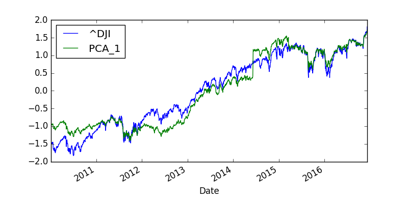
There is difference. You can see PCA_1 is following Dow Jones index by there is some difference. Since the first component is only explaining 63% of the variability we don’t expect it to follow Dow Jones very closely. We should include the first 5 PCA components into PCA_5 and see how well it follows the Dow Jones. We plot the 3 lines PCA_1, PCA_5 and DJIA and see how well these 2 PCA indexes approximate DJIA.
#improve the results

pca = KernelPCA(n_components=5).fit(data.apply(scale_function))

pca_components = pca.transform(-data)

weights = get_we(pca.lambdas_)

dji['PCA_5'] = np.dot(pca_components, weights)
import matplotlib
import matplotlib.pyplot as plt
dji.apply(scale_function).plot(figsize=(8, 4))
Below is the plot of the three lines on the same graph!
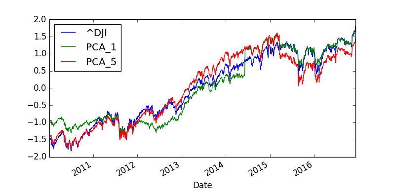
There is some difference still. Anyway the purpose of this post was only educational. We wanted to show how to do PCA on Dow Jones Index.