In this post we are going to develop ARIMA and GARCH model for S&P500 weekly time series. S&P 500 is a very popular US stock market index and is considered to be a barometer of US economy. It is a capitalization weighted index of 500 US stocks representing different business sectors in the US economy. S&P stands for Standard & Poor’s. Did you read the post on S&P 500 Death Cross? S&P 500 daily and weekly data is heavily studied by the analysts for clues on US stock market behavior.There are many traders who love to trade this stock market index. If we can successfully predict the direction of this stock market index, we can make a lot of money. The question is can we really predict the direction and volatility of this index? We will try to answer this question in this post. Watch this 50 minute documentary on NY Stock Exchange Flash Crash. Okay let’s start our discussion! This ARIMA Plus GARCH Trading Strategy can be used for any stock. You can use this strategy to trade Apple, Google, Facebook, Microsoft or any other stock alongwith stock market indices like Dow Jones, FTSE 100 etc.The basic idea is to predict the return and volatility for the next week. If the predicted return is positive, we will open a long position and if the predicted return is negative we will open a short position.
Downloading S&P 500 Weekly Data
First we need to download S&P 500 weekly data. We will download S&P 500 data from Yahoo Finance. We can download the daily data of any stock using Quantmod R package This daily data is already formatted in required xts object. Then we use the to.weekly command to easily convert the data to weekly data. Did you read the post on how to do Principal Component Analysis of Dow Jones Index? Below is the R code that accomplishes this. We will download the data from January 2010 to January 2017. When it comes to time series analysis, R is much more powerful as compared to Python. Python still lacks the elegance of R when it comes to doing time series analysis. R and Python are two powerful languages if you want to master machine learning and artificial intelligence.
> #download S&P 500 Daily and Weekly data from Yahoo Finance
> #load library
> library(quantmod)
> #create an environment
> sp500 <- new.env()
> #first we download the daily time series data from Yahoo Finance
> getSymbols("^GSPC", env = sp500, src = "yahoo",
+            from = as.Date("2010-01-04"), to = as.Date("2017-02-01"))
[1] "GSPC"
Warning message:
In download.file(paste(yahoo.URL, "s=", Symbols.name, "&a=", from.m,  :
  downloaded length 143315 != reported length 200
> GSPC1 <- sp500$GSPC
> head(GSPC1)
           GSPC.Open GSPC.High GSPC.Low GSPC.Close GSPC.Volume GSPC.Adjusted
2010-01-04   1116.56   1133.87  1116.56    1132.99  3991400000       1132.99
2010-01-05   1132.66   1136.63  1129.66    1136.52  2491020000       1136.52
2010-01-06   1135.71   1139.19  1133.95    1137.14  4972660000       1137.14
2010-01-07   1136.27   1142.46  1131.32    1141.69  5270680000       1141.69
2010-01-08   1140.52   1145.39  1136.22    1144.98  4389590000       1144.98
2010-01-11   1145.96   1149.74  1142.02    1146.98  4255780000       1146.98
> class(GSPC1)
[1] "xts" "zoo"
> dim(GSPC1)
[1] 1783    6
> # Plot the daily price series and volume
> chartSeries(GSPC1,theme="white")
> #convert the data to weekly
> GSPC2 <-to.weekly(GSPC1)
> head(GSPC2)
           GSPC1.Open GSPC1.High GSPC1.Low GSPC1.Close GSPC1.Volume GSPC1.Adjusted
2010-01-08    1116.56    1145.39   1116.56     1144.98  21115350000        1144.98
2010-01-15    1145.96    1150.41   1131.39     1136.03  21816230000        1136.03
2010-01-22    1136.03    1150.45   1090.18     1091.76  22618329600        1091.76
2010-01-29    1092.40    1103.69   1071.59     1073.87  25397670000        1073.87
2010-02-05    1073.89    1104.73   1044.50     1066.19  25411190000        1066.19
2010-02-12    1065.51    1080.04   1056.51     1075.51  22017080000        1075.51
> dim(GSPC2)
[1] 370   6
> # Plot the weekly price series and volume
> chartSeries(GSPC2,theme="white")
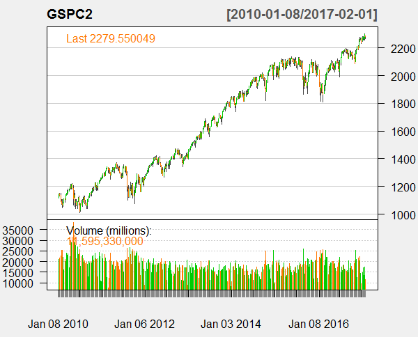
We have 370 observations in our data frame. You can also read the post on how to download the stock market daily data from Yahoo Finance using Python Pandas Module.Below is the plot of the weekly data. In the plot below you can see S&P 500 index has been on an upward trajectory during the period 2010 and 2017.
Fitting An ARIMA Model To S&P 500 Weekly Data
ARIMA stands for Autoregressive Integrated Moving Average. In ARIMA we combine the autoregressive model with moving average model while differencing the time series. The challenge lies in finding the correct order of ARIMA model. You should be familiar with what is an ARIMA model. If you have no idea what ARIMA is, you can watch this video below that explains what ARIMA model is. After watching this video you can continue to read the rest of the post.The video below explains in detail what is AR, MA, ARMA and ARIMA model.
First we take the logarithm of the closing price. After that we difference the time series. Differencing the log of the closing price gives the price return series. First we remove the NAs. After that we difference the log series. Differencing converts the log series to a return series. In financial time series analysis literature the focus is on the return and volatility which is the standard deviation of the return series.
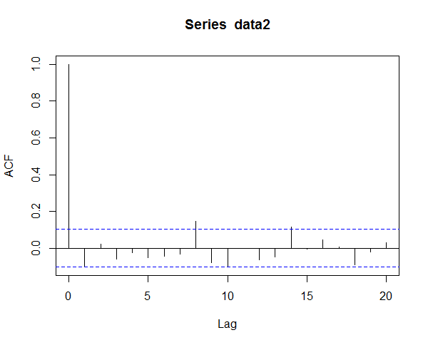
> ##ARIMA model for S&P 500 Weekly Time Series
> #First we take the log of the closing price
> data1 <- log(GSPC2$GSPC1.Close)
> #plot the log series
> chartSeries(data1,theme="white")
> #plot autocorrelation function upto 20 lags
> acf(data1,lag=20)
> #difference the weekly time series
> data2 <- diff(data1)
> data2 <- data2[!is.na(data2)]
> library(fBasics)
> basicStats(data2)
            GSPC1.Close
nobs         369.000000
NAs            0.000000
Minimum       -0.074603
Maximum        0.071284
1. Quartile   -0.007677
3. Quartile    0.013454
Mean           0.001866
Median         0.002826
Sum            0.688591
SE Mean        0.001038
LCL Mean      -0.000175
UCL Mean       0.003907
Variance       0.000398
Stdev          0.019941
Skewness      -0.432273
Kurtosis       1.612349
> #plot autocorrelation function upto 20 lags
> acf(data2,lag=20)
> #plot the partial autocorrelation function upto 20 lags
> pacf(data2,lag=20)
In the above code you can see that we have 369 observations in our weekly data. The returns data is skewed and has a high kurtosis. Read this post that explains how to buy your favorite stock at a much lower price. The important thing is to determine the order (p, d,q) of ARIMA model. One method is to use the autocorrelation function and the partial autocorrelation function. Below is the plot of the return series autocorrelation function (ACF) and partial autocorrelation function(PCF). Second method is to use the Akaike Information Criterion (AIC) and try to iterate through different values of p and q and see which combination reduces the AIC.
This is the Partial Autocorrelation Function (PCF).
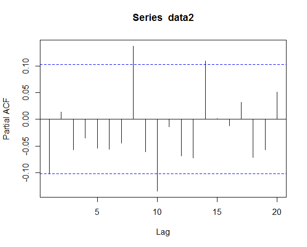
In the above plot you can see that there is autocorrelation between lags. However, here we will however use a different approach given in the book,”An Introduction to Analysis Of Financial Time Series Using R” , by Tsay. He calls it Extended Autocorrelation Function (EACF).
> library(TSA)
> m7<-eacf(data1,20,20)
AR/MA
   0 1 2 3 4 5 6 7 8 9 10 11 12 13 14 15 16 17 18 19 20
0  x x x x x x x x x x x  x  x  x  x  x  x  x  x  x  x
1  o o o o o o o x o o o  o  o  x  o  o  o  o  o  o  o
2  x o o o o o o x o x o  o  o  x  o  o  o  o  o  o  o
3  x x o o o o o o o x o  o  o  x  o  o  o  o  o  o  o
4  x x x o o o o o o o o  o  o  x  o  o  o  o  o  o  o
5  x x o o o o o o o o o  o  o  o  o  o  o  o  o  o  o
6  x x o o o o o o o x o  o  o  o  o  o  o  o  o  o  o
7  x o o x x x o o o x o  o  o  o  o  o  o  o  o  o  o
8  x x x o o x o o o x x  o  o  o  o  o  o  o  o  o  o
9  x x x o o x x x o x x  o  o  o  o  o  o  o  o  o  o
10 x x x x o x x x o x o  o  o  o  o  o  o  o  o  o  o
11 o x x x x x o o o o o  o  o  o  o  o  o  o  o  o  o
12 o x x x x o o o o o x  o  o  o  o  o  o  o  o  o  o
13 x x x x x x o o o o x  o  o  o  o  o  o  o  o  o  o
14 x x x x x o x o o o x  x  o  o  o  o  o  o  o  o  o
15 x o x x x x x o o o o  o  o  o  o  o  o  o  o  o  o
16 x o x x o x o o o x o  o  o  o  x  o  o  o  o  o  o
17 x x o x o x x x o x o  o  o  o  x  o  o  o  o  o  o
18 x x x x o x o x x o o  o  o  o  o  o  o  o  o  o  o
19 x x x o o x o o x o o  o  o  o  x  o  o  o  o  o  o
20 x x o x x x o o o o o  o  o  x  x  x  o  o  o  o  o
From the above we can see there are no moving average shocks. We start by trying an Autoregressive Model of order 20 also abbreviated with AR(20). R takes less than a minute to do all the calculations. I have reproduced the calculations below.
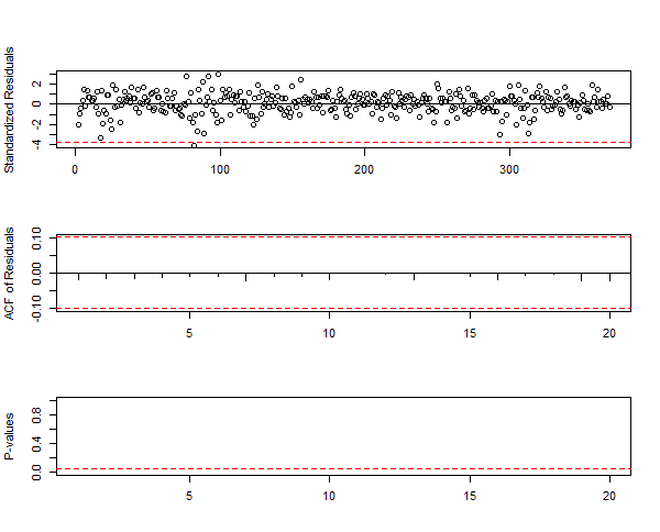
> #fit an ARIMA model to the weekly time series
> m2 <- arima(data2,order=c(20,0,0),include.mean=F)
> m2

Call:
arima(x = data2, order = c(20, 0, 0), include.mean = F)

Coefficients:
          ar1     ar2      ar3      ar4      ar5      ar6      ar7    ar8      ar9
      -0.0811  0.0484  -0.0630  -0.0019  -0.0196  -0.0874  -0.0143  0.153  -0.0757
s.e.   0.0519  0.0522   0.0521   0.0520   0.0522   0.0523   0.0518  0.052   0.0528
         ar10    ar11     ar12     ar13    ar14    ar15    ar16    ar17     ar18
      -0.1004  0.0197  -0.0744  -0.0438  0.1356  0.0149  0.0092  0.0545  -0.0610
s.e.   0.0526  0.0528   0.0527   0.0521  0.0521  0.0526  0.0527  0.0535   0.0534
         ar19    ar20
      -0.0354  0.0727
s.e.   0.0537  0.0535

sigma^2 estimated as 0.0003647:  log likelihood = 936.53,  aic = -1833.05
> tsdiag(m2,gof=20)
You can see in the above summary ar14 coefficient is quite high. It is even higher than ar1 coefficient. We can further prune this model and remove some ar coefficients but there is no harm in using the above model as it is. So we make the forecast now. before we do that I have also printed the Box-Ljung test. This test tells us whether any autocorrelation is different from zero.
> Box.test(m2$residuals,lag=20,type='Ljung')

	Box-Ljung test

data:  m2$residuals
X-squared = 1.5565, df = 20, p-value = 1
> #make the next predict
> pred1 <- predict(m2, n.ahead=5)
> pred1
$pred
Time Series:
Start = 370
End = 374
Frequency = 1
[1] -0.0036807128 -0.0003242848 -0.0002981998  0.0024376336  0.0002359116

$se
Time Series:
Start = 370
End = 374
Frequency = 1
[1] 0.01909728 0.01915997 0.01918870 0.01923712 0.01923840
Fitting A GARCH Model To S&P 500 Weekly Time Series
We will fit a GARCH(1,1) model to S&P 500 weekly time series. In most book GARCH(1,1) model has been considered to be adequate to modelling a financial time series. Higher order GARCH models can take longer time to calculate. R takes a few seconds to calculate GARCH(1,1) model. Did you read the post on how I made $500K in 1 year with machine learning and high frequency trading? If you have no idea what is this GARCH model, you should watch the video below. I will not go into the theory of GARCH Modelling. GARCH stands for Generalized Autoregressive Conditional Heteroscedastic.Volatility of a financial return series is just the standard deviation of the return series. If you are interested in knowing theory behind GARCH, you can watch the video below that explains things in detail.
Now as said above, GARCH(1,1) is adequate for our modelling. Below I have provided the R code for doing the modelling. I have made 3 models. First model uses Gaussian residuals. Second model uses Student t Distribution residuals. Third model uses Skewed Student t Distribution residuals. Financial time series are fat tailed. In the beginning of this post, I have provided the basic summary for the weekly return series. You can check it is skewed and has significant kurtosis.
> #Fit a GARCH(1,1) model
> library(fGarch)
> m4=garchFit(~1+garch(1,1),data=data2,trace=F)
> summary(m4)

Title:
 GARCH Modelling

Call:
 garchFit(formula = ~1 + garch(1, 1), data = data2, trace = F)

Mean and Variance Equation:
 data ~ 1 + garch(1, 1)
<environment: 0x000000000e5ff4a0>
 [data = data2]

Conditional Distribution:
 norm

Coefficient(s):
        mu       omega      alpha1       beta1
2.7309e-03  4.6625e-05  1.8094e-01  6.9924e-01

Std. Errors:
 based on Hessian

Error Analysis:
        Estimate  Std. Error  t value Pr(>|t|)
mu     2.731e-03   8.764e-04    3.116  0.00183 **
omega  4.663e-05   1.806e-05    2.582  0.00982 **
alpha1 1.809e-01   5.701e-02    3.174  0.00151 **
beta1  6.992e-01   8.038e-02    8.700  < 2e-16 ***
---
Signif. codes:  0 ‘***’ 0.001 ‘**’ 0.01 ‘*’ 0.05 ‘.’ 0.1 ‘ ’ 1

Log Likelihood:
 946.8713    normalized:  2.566047

Description:
 Sun Feb 19 17:59:13 2017 by user: ahmad


Standardised Residuals Tests:
                                Statistic p-Value
 Jarque-Bera Test   R    Chi^2  22.53862  1.275855e-05
 Shapiro-Wilk Test  R    W      0.9853689 0.0008688758
 Ljung-Box Test     R    Q(10)  13.78564  0.1829956
 Ljung-Box Test     R    Q(15)  17.23394  0.305073
 Ljung-Box Test     R    Q(20)  21.54706  0.3655851
 Ljung-Box Test     R^2  Q(10)  9.803976  0.4578563
 Ljung-Box Test     R^2  Q(15)  13.75911  0.5438716
 Ljung-Box Test     R^2  Q(20)  18.79287  0.5353239
 LM Arch Test       R    TR^2   10.89109  0.538275

Information Criterion Statistics:
      AIC       BIC       SIC      HQIC
-5.110414 -5.068020 -5.110645 -5.093573

> #calculate volatility
> v1=volatility(m4)
> #standardize the residuals
> resi=residuals(m4,standardize=T)
> vol=ts(v1,frequency=52,start=c(2010,2))
> res=ts(resi,frequency=52,start=c(2010,2))
> #Show volatility and residuals
> par(mfcol=c(2,1))
> plot(vol,xlab='year',ylab='volatility',type='l')
> plot(res,xlab='year',ylab='st. resi',type='l')
> # Obtain ACF & PACF
> par(mfcol=c(2,2))
> acf(resi,lag=24)
> pacf(resi,lag=24)
> acf(resi^2,lag=24)
> pacf(resi^2,lag=24)
> #fit Student t innovations
> m5 <-garchFit(~1+garch(1,1),data=data2,trace=F,cond.dist="std")
> summary(m5)

Title:
 GARCH Modelling

Call:
 garchFit(formula = ~1 + garch(1, 1), data = data2, cond.dist = "std",
    trace = F)

Mean and Variance Equation:
 data ~ 1 + garch(1, 1)
<environment: 0x000000000ec6cbf8>
 [data = data2]

Conditional Distribution:
 std

Coefficient(s):
        mu       omega      alpha1       beta1       shape
2.9737e-03  4.4679e-05  1.7147e-01  7.1428e-01  8.0282e+00

Std. Errors:
 based on Hessian

Error Analysis:
        Estimate  Std. Error  t value Pr(>|t|)
mu     2.974e-03   8.650e-04    3.438 0.000587 ***
omega  4.468e-05   2.007e-05    2.226 0.025997 *
alpha1 1.715e-01   6.466e-02    2.652 0.008005 **
beta1  7.143e-01   9.109e-02    7.841 4.44e-15 ***
shape  8.028e+00   3.331e+00    2.410 0.015953 *
---
Signif. codes:  0 ‘***’ 0.001 ‘**’ 0.01 ‘*’ 0.05 ‘.’ 0.1 ‘ ’ 1

Log Likelihood:
 951.122    normalized:  2.577566

Description:
 Sun Feb 19 17:59:14 2017 by user: ahmad


Standardised Residuals Tests:
                                Statistic p-Value
 Jarque-Bera Test   R    Chi^2  22.74551  1.150471e-05
 Shapiro-Wilk Test  R    W      0.9852331 0.000806252
 Ljung-Box Test     R    Q(10)  13.84592  0.1801365
 Ljung-Box Test     R    Q(15)  17.33     0.2995226
 Ljung-Box Test     R    Q(20)  21.6582   0.3593419
 Ljung-Box Test     R^2  Q(10)  9.735707  0.4639787
 Ljung-Box Test     R^2  Q(15)  13.74266  0.5451293
 Ljung-Box Test     R^2  Q(20)  18.72744  0.5396011
 LM Arch Test       R    TR^2   10.94489  0.5336479

Information Criterion Statistics:
      AIC       BIC       SIC      HQIC
-5.128032 -5.075041 -5.128393 -5.106981

> v2 <-volatility(m5)
> #fit Skew Student t innovations
> m6 <-garchFit(~1+garch(1,1),data=data2,trace=F,cond.dist='sstd')
> summary(m6)

Title:
 GARCH Modelling

Call:
 garchFit(formula = ~1 + garch(1, 1), data = data2, cond.dist = "sstd",
    trace = F)

Mean and Variance Equation:
 data ~ 1 + garch(1, 1)
<environment: 0x0000000010e862d0>
 [data = data2]

Conditional Distribution:
 sstd

Coefficient(s):
        mu       omega      alpha1       beta1        skew       shape
2.5839e-03  4.0451e-05  1.6163e-01  7.2921e-01  8.5054e-01  9.3662e+00

Std. Errors:
 based on Hessian

Error Analysis:
        Estimate  Std. Error  t value Pr(>|t|)
mu     2.584e-03   8.855e-04    2.918  0.00352 **
omega  4.045e-05   1.891e-05    2.139  0.03240 *
alpha1 1.616e-01   6.029e-02    2.681  0.00734 **
beta1  7.292e-01   9.004e-02    8.099 6.66e-16 ***
skew   8.505e-01   6.275e-02   13.554  < 2e-16 ***
shape  9.366e+00   4.475e+00    2.093  0.03636 *
---
Signif. codes:  0 ‘***’ 0.001 ‘**’ 0.01 ‘*’ 0.05 ‘.’ 0.1 ‘ ’ 1

Log Likelihood:
 953.6572    normalized:  2.584437

Description:
 Sun Feb 19 17:59:15 2017 by user: ahmad


Standardised Residuals Tests:
                                Statistic p-Value
 Jarque-Bera Test   R    Chi^2  23.36055  8.459041e-06
 Shapiro-Wilk Test  R    W      0.9849739 0.0006994371
 Ljung-Box Test     R    Q(10)  13.74952  0.1847262
 Ljung-Box Test     R    Q(15)  17.25512  0.3038433
 Ljung-Box Test     R    Q(20)  21.55964  0.3648753
 Ljung-Box Test     R^2  Q(10)  9.096845  0.522938
 Ljung-Box Test     R^2  Q(15)  12.91374  0.6089609
 Ljung-Box Test     R^2  Q(20)  17.57954  0.6150844
 LM Arch Test       R    TR^2   10.17462  0.6006445

Information Criterion Statistics:
      AIC       BIC       SIC      HQIC
-5.136354 -5.072763 -5.136871 -5.111092

>
>
> #plot the 3 models
> v3=volatility(m6)
> plot(v3)
> predictedVolatility <- predict(m6, n.ahead = 1)
> predictedVolatility
  meanForecast  meanError standardDeviation
1  0.002583897 0.01438093        0.01438093
In the above code we have fitted three models. Read the post on how to build a Quantitative Trading Strategy that beats S&P 500. Below is the plot of the GARCH(1,1) modell m4. This is the Gaussian residuals model. Now I was surprised at the speed with which R calculated the 3 different GARCH models. I would prefer the third model as it introduced skewness into out model with tails that are fatter than the normal distribution.
Now that we have the one step ahead return and volatility we can make our prediction. One step ahead return prediction -0.0036 and the volatility is 0.00258. So the predicted upper bound and the lower bound of predicted return is: 0.001456 and -0.00865. So essentially this is the limit in which the return will be. We can use some filter like a minimum return value before we enter into a long or a short trade. We can also use this strategy for daily trading instead of weekly trading. In future posts we will go into this strategy in more depth.