Options trading has become very popular in recent years. Did you read the post on how to get paid for buying your favorite stock? In this post you learn an options trading strategy that you can use to buy your favorite stock at a lower price. Options are a type of derivatives. Derivatives have been hailed as the financial revolution of the late 20th century. Derivatives types are forwards, futures, swaps and options. Derivatives are instruments that derive their value from another underlying asset. In the case of stock options, their prices depend on the underlying stock.
In this post first we will build two options pricing models. The first one is the famous Black Scholes Options pricing model and the second one is the Cox-Ross-Rubinstein Options pricing model. After that we will also discuss what options greeks are and how to model implied volatility. We will also discuss why in practice both these options pricing formulas are used in reverse to calculate implied volatility instead of options price. . We will be using R for doing the analysis. You should have installed R and RStudio. I would suggest if you fast a very fast implementation, you should install Microsoft R Open. Quantmod is an important R package that provides technical analysis. Read this post on how to use R package Quantmod in daily stock market analysis.
Options as said above drive their value from the underlying stock. The problem is we don’t know whether the options contract is going to be exercised or not. This brings a level of complexity when we try to price the stock options contract. Black Scholes formula assumes a continuous stochastic process while Cox-Ross-Rubinstein model assumes a discrete stochastic process. So let’s start with Black Scholes Options pricing formula. Read this post on fail safe EMA trading system.
Black Scholes Stock Options Pricing Formula
Black Scholes options pricing formula makes a few assumptions. The first is market is arbitrage free. This means that there is no price differential possible. The second assumption is that the underlying asset price follows a Brownian motion. The third assumptions says that the underlying stock does not pay any dividend.. Fourth assumption is that there are no transaction costs involved and buying and selling of the underlying stock can be done in any fractional amount. The last assumption is that we know the short term interest rate and this interest rate is constant over time. Now we don’t need to go into the details of how we derive this formula mathematically. We will use R for calculating the stock options price when we know the different parameters used in calculating the stock options price. Below we use R to calculate Apple AAPL stock call option price with expiry 3 months. Apple AAPL stock price is $130 and the stock options contract strike price is $140.
> library(fOptions)
Loading required package: timeDate
Loading required package: timeSeries
Loading required package: fBasics


Rmetrics Package fBasics
Analysing Markets and calculating Basic Statistics
Copyright (C) 2005-2014 Rmetrics Association Zurich
Educational Software for Financial Engineering and Computational Science
Rmetrics is free software and comes with ABSOLUTELY NO WARRANTY.
https://www.rmetrics.org --- Mail to: info@rmetrics.org


Rmetrics Package fOptions
Pricing and Evaluating Basic Options
Copyright (C) 2005-2014 Rmetrics Association Zurich
Educational Software for Financial Engineering and Computational Science
Rmetrics is free software and comes with ABSOLUTELY NO WARRANTY.
https://www.rmetrics.org --- Mail to: info@rmetrics.org
> GBSOption(TypeFlag = "c", S = 130, X =140, Time = 1/4, r = 0.02,
+           sigma = 0.22, b = 0.02)

Title:
 Black Scholes Option Valuation

Call:
 GBSOption(TypeFlag = "c", S = 130, X = 140, Time = 1/4, r = 0.02,
     b = 0.02, sigma = 0.22)

Parameters:
          Value:
 TypeFlag c
 S        130
 X        140
 Time     0.25
 r        0.02
 b        0.02
 sigma    0.22

Option Price:
 2.382111

Description:
 Sun May 07 18:12:25 2017
First we load the fOptions library, c means call option.S is the stock price which is $130 per share. X is the stock options strike price which is $140 per share. Short term interest rate is 2%. Implied volatility has been assumed to be 22%. Apple stock call option price is $2.38. This is how it works. Apple stock right now is trading at $130 per share. We buy a call option. We believe Apple stock price will increase so we buy a call options with 3 month expiry on Apple stock with strike price of $140. If price goes above $140 we can buy the AAPL stocks at $140 per share. Right now Apple stock is trading at $148 per share. So you can see we can buy Apple stock cheap. We will exercise the Apple stock call options contract at $140 and then sell the stock in the market for $148 making a profit of $8 per share. Since the price was $2.38 per 100 shares we make a good profit. Read this post on a Keltner Chanels trading strategy that made $1.1 million. Suppose our strike price was $135.
> GBSOption(TypeFlag = "c", S = 130, X =135, Time = 1/4, r = 0.02,
+           sigma = 0.22, b = 0.02)

Title:
 Black Scholes Option Valuation

Call:
 GBSOption(TypeFlag = "c", S = 130, X = 135, Time = 1/4, r = 0.02,
     b = 0.02, sigma = 0.22)

Parameters:
          Value:
 TypeFlag c
 S        130
 X        135
 Time     0.25
 r        0.02
 b        0.02
 sigma    0.22

Option Price:
 3.88815

Description:
 Sun May 07 18:22:29 2017
In this case stock options price has increased to $3.88. Now as said above we don’t need to know how to derive this Black Scholes Options pricing formula. We just need to plug-in the different parameters in the formula like call/put option, stock price, strike price, short term interest rate, implied volatility etc. Now the problem is we don’t have any way to calculate implied volatility. We just assumed an implied volatility formula. If you don’t know what are the different parameters are use the following formula.
> str(GBSOption)
function (TypeFlag = c("c", "p"), S, X, Time, r, b, sigma, title = NULL, description = NULL)
We can also calculate put options price . It is also very easy when using R. Below is a put option price calculation. We changed c to p in the formula. Apple stock price is $130. Put option strike price is $135. Expiry is 3 months. Short term interest rate is 2%. Implied volatility is 22%.
> GBSOption(TypeFlag = "p", S = 130, X =135, Time = 1/4, r = 0.02, sigma
+           = 0.22, b = 0.02)@price
[1] 8.214834
Now as said above Black Scholes Options pricing formula depends on implied volatility a lot. Implied volatility is something we don’t know. So practically we can’t use this Black Scholes Stock Options price formula. Most of the time we use the formula in reverse. We plugin in the stock option price in the formula and calculate implied volatility. We can use the GARCH model to calculate volatility. Read this post on how to use GARCH in trading.
The Cox-Ross-Rubinstein Stock Options Pricing Formula
Cox-Ross-Rubinstein formula also known as CRR formula is different from Black Scholes Stock Options pricing formula. The fundamental assumption in CRR formula is that the underlying stock price follows a discrete binomial distribution. What this means is that stock price either moves up by a certain amount or moves down by a certain amount in each period. The binomial tree is recombining. What this means is that in 2 periods, price can go up and then down or it can go down and up with the same end price. Below is calculate Apple stock options price using the same strike price, implied volatility, short term interest rate as above for Black Scholes formula.
> CRRBinomialTreeOption(TypeFlag = "ce", S = 130, X = 135,
+                       Time = 1/4, r = 0.02, b = 0.02, sigma = 0.22, n = 3)@price
[1] 4.033903
> CRRBinomialTreeOption(TypeFlag = "pe", S = 130, X = 135,
+                       Time = 1/4, r = 0.02, b = 0.02, sigma = 0.22, n = 3)@price
[1] 8.360588
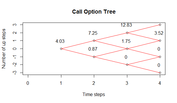
You can see options prices using Cox-Ross-Rubinstein formula are close to Black Scholes formula but not the same.Now don’t need to do the complex mathematical derivation of the CRR formula. We can also plot the above call options formula as well the put options formula binomial tree for 3 periods.Below is the code for call options binomial tree.
> CRRTree <- BinomialTreeOption(TypeFlag = "ce", S = 130, X = 135,
+                               Time = 1/4, r = 0.02, b = 0.02, sigma = 0.22, n = 3)
> BinomialTreePlot(CRRTree, dy = 1, xlab = "Time steps",
+                  ylab = "Number of up steps", xlim = c(0,4))
> title(main = "Call Option Tree")
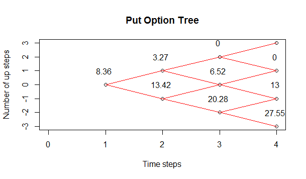
By changing ce to pe we can also plot the put options binomial tree. Read this post on how to do Principle Component Analysis on Dow Jones Industrial Average DJIA.Below is the call options binomial tree plot.
Below is the put options binomial tree.
Now you saw a difference in options price between the both formulas. The price difference is not much. Black Scholes calculated call options price as $3.88 while Cox-Ross-Rubinstein formula calculated call options price as $4.03. The difference is not great but it is there. It is due to the difference in the two formulas mathematical derivations. In Black Scholes formula we assume a continuous stochastic formula while in Cox-Ross-Rubinstein formulas assumes a discrete binomial formula. W can reduce the price difference by reducing the length of the time step in Cox-Ross-Rubinstein formula.
How To Calculate Options Greeks?
Greeks measure sensitivity of an options contract to different market factors. For example delta is the sensitivity to underlying stock price. Gamma is the sensitivity to delta to underlying stock price. You can call gamma delta of delta. Theta is sensitivity to time while rho is sensitivity to risk free rate. Lastly vega is the sensitivity to implied volatility. In mathematical terms all the greeks are partial derivatives that measure the rate of change with respect to some parameter. Below we calculate the greeks using R.
> sapply(c('delta', 'gamma', 'vega', 'theta', 'rho'), function(greek)
+   GBSGreeks(Selection = greek, TypeFlag = "c", S = 130, X = 135,
+             Time = 1/4, r = 0.02, b = 0.02, sigma = 0.22))
      delta       gamma        vega       theta         rho
  0.4041424   0.0270888  25.1790377 -12.0517840  12.1625922
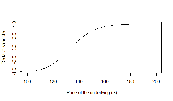
You can see R is very fast in calculating the greeks. Straddle is an important options trading strategy. We construct a stradde by buying a put and a call option at the same time. Below is the delta calculations for a straddle.
> straddles <- sapply(c('c', 'p'), function(type) sapply(100:200, function(S)
+   GBSGreeks(Selection = 'delta', TypeFlag = type, S = S,
+             X = 135, Time = 1/4, r = 0.02, b = 0.02, sigma = 0.22)))
> plot(100:200, rowSums(straddles), type='l',
+      xlab='Price of the underlying (S)', ylab = 'Delta of straddle')
Econometrics is an important subject that many traders don’t know. I have developed this course on Econometrics for Traders in which I show you how you can use econometrics in your trading.Below is the delta plot for this straddle option build with Apple stock put and call options.
If you are interested, you can take a look at my course Stochastic Calculus for Traders. In this course, I show you how to mathematically derive Black Scholes options pricing formula as well as Cox-Ross-Rubinstein options pricing formula.